Visualizing field files
OpenFTS field files can be visualized a few different ways by using the
fieldkit library located here.
In this tutorial, we will visualize density field files using each method
available. To begin enter a directory containing OpenFTS and your field file,
which in this tutorial will be named density.dat and correspond to a gyroid
phase.
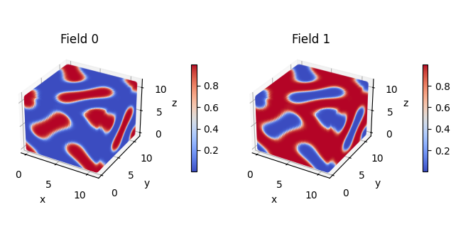
With matplotlib.pyplot
This is the best method for quickly visualizing field files. To do so, we run the following in python:
import fieldkit as fk
density_fields = fk.read_from_file('density.dat')
fk.plot(fields=density_fields, show=True)
For common operations like these, fieldkit has standalone scripts that can
be executed from the command line to accomplish the same task.
$ OpenFTS/extern/fieldkit/tools/fk_plot.py density.dat
With visual molecular dynamics (VMD)
For more control over your visualizations you can use
VMD. We first use fieldkit to
convert the field file to the
cube file format.
import fieldkit as fk
density_fields = fk.read_from_file('density.dat')
fk.write_to_cube_files(prefix='density', fields=density_fields)
Alternatively we can run the following from the command line:
$ OpenFTS/extern/fieldkit/tools/fk_convert_to_cube.py density.dat
This generates a cube file per field in the field file. Let’s now visualize the first field.
$ vmd density_field0.cube
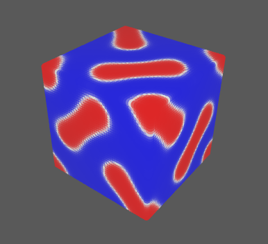
fieldkit labels each voxel as an atom in the cube file in addition to
converting the field data to volumetric data. We can therefore either
visualize the voxels themselves:
vmd > mol rep Points 20
vmd > mol color Charge
vmd > mol addrep 0
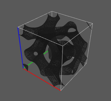
Or visualize the volumetric data by computing isosurfaces, where here we set the isovalue to 0.75.
vmd > mol rep Isosurface 0.75 0 3 1 1 1
vmd > mol color ColorID 16
vmd > mol addrep 0
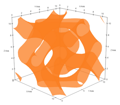
With paraview
For the greatest control over your visualizations you can use
paraview. First we use fieldkit to convert
the field file to a VTK file.
import fieldkit as fk
density_fields = fk.read_from_file('density.dat')
fk.write_to_VTK(filename='density.vtk', fields=density_fields)
We can also alternatively do so from the command line.
$ OpenFTS/extern/fieldkit/tools/fk_convert_to_vtk.py density.dat
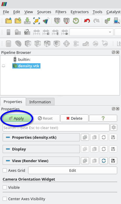
This generates density.vtk which we can visualize with paraview.
$ paraview density.vtk
Like VMD, paraview can also compute isosurfaces as well as other sophisticated
visualizations. To compute the same isosurface as we did in VMD, first we must
apply the density.vtk file.
Next we have to configure the isosurface and make the axes visible.
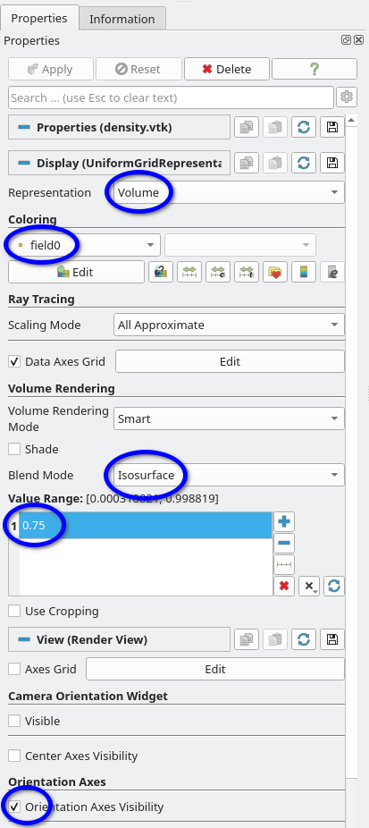
And now we have a visualization of the gyroid phase. Something to keep in mind:
as your total number of plane waves increase for your fts object,
interacting with the visualization can become slow. For high numbers of plane
waves, we find that paraview gives the best performance.