SCFT/FTS Basics

Now that you know how to build, run, and analyze lets put it all together and actually run some simulations.

In this example, we will consider a FTS workflow where we:

1. Run an initial 1D SCFT simulation to determine the equilibrium box length

2. Convert these 1d fields into 3d fields using fieldkit

3. Initialize a new simulation from these 3d fields and run a complex Langevin (CL) simulation

For this example we will be running OpenFTS as a python package.

1D Variable Cell SCFT

Our first step is to setup a 1d SCFT simulation. We will first import the openfts package and create a fts object

import openfts

Now we will setup our simulation parameters. An explanation of these parameters are covered in more detail in Simulation Setup.

# create an OpenFTS object
fts = openfts.OpenFTS()

# initialize the cell
fts.cell(cell_scale=1.0,cell_lengths=[4.3],dimension=1,length_unit='Rg')

# initialize the fields to use 32 grid points
fts.field_layout(npw=[32],random_seed=1)

# initialize the driver (including the field updater and variable cell)
fts.driver(dt=5.0,nsteps=4000,output_freq=50,type='SCFT',stop_tolerance=1e-05,)
fts.field_updater(type='EMPEC',update_order='simultaneous',adaptive_timestep=False,lambdas=[1.0, 1.0])
fts.variable_cell(lambda_=0.2,stop_tolerance=0.0001,update_freq=20,shape_constraint='none')

# number of beads in chain
N = 50

# Create the model with chiN=20 and BC=100
fts.model(type='MeltChiAB', Nref=N,bref=1.0,chiN=20.,inverse_BC=0.01)

# initialize the model fields
# mu_minus is initialized with a gaussian centered at zero, mu_plus is random
fts.init_model_field(fieldname='mu_minus',type='gaussians', height=1.0,ngaussian=1,width=0.1,centers=[0])
fts.init_model_field(fieldname='mu_plus',type='random',mean=0.0,stdev=1.0)

# create a molecule, here a diblock consisting of N beads with fA=0.5
fts.add_molecule(type='PolymerLinear',chain_type='discrete',
                 nbeads=N,nblocks=2,block_fractions=[0.5, 0.5],block_species=['A', 'B'],
                 volume_frac=1.0)

# Set the operators we seek to output
# for SCFT the Hamiltonian and CellStress are sufficient
fts.add_operator(averaging_type='none',type='Hamiltonian')
fts.add_operator(averaging_type='none',type='CellStress')

# Use the default names of output files
fts.output_default()

# Use two species types A and B, each with a smearing length of 0.15 Rg
fts.add_species(label='A',stat_segment_length=1.0, smearing_length=0.15)
fts.add_species(label='B',stat_segment_length=1.0, smearing_length=0.15)

Now we’re ready to run OpenFTS

fts.run()

============================================================
                          OpenFTS

OpenFTS version: heads/develop 1e8cdcf DIRTY
FieldLib version: heads/master e7d9bf6 CLEAN
Execution device: [CPU]
FieldLib precision: double
=============================================================

Initialize Cell
  * dim = 1
  * length unit = Rg
  * cell_lengths = [4.300000 ]
  * cell_tensor:
4.3
Initialize FieldLayout
  * npw = [32 ]
  * random_seed = 1
Initialize Species
  * label = A
  * stat_segment_length = 1.000000
  * smearing_length = 0.150000
  * charge = 0.000000
Initialize Species
  * label = B
  * stat_segment_length = 1.000000
  * smearing_length = 0.150000
  * charge = 0.000000
Initialize ModelMeltChiAB
  * bref = 1
  * Nref = 50
  * chiN = 20
  * compressibility_type = exclvolume
  * inverse_BC = 0.01
  * initfields = yes
                 using gaussians
Initialize MoleculePolymerLinear
  * volume_frac = 1
  * chain_type = discrete
  * Linear polymer has single chain:
    - type = discrete
    - nbeads = 50
    - discrete_type = Gaussian
    - sequence_type = blocks
    - nblocks = 2
    - block_fractions =  0.500000 0.500000
    - block_species =  A B
    - monomer_sequence (compact) =  A_25 B_25
    - monomer_sequence (long) = AAAAAAAAAAAAAAAAAAAAAAAAABBBBBBBBBBBBBBBBBBBBBBBBB
Initialize DriverSCFTCL
  * is_complex_langevin = false
  * dt = 5.000000
  * output_freq = 50
  * block_size = 50
  * field_updater = EMPEC
    - adaptive_timestep = false
    - predictor_corrector = true
    - update_order = simultaneous
    - lambdas = 1.000000 1.000000
  * field_stop_tolerance = 1e-05
  * variable_cell enabled:
    - cell_lambda = 0.2
    - cell_stop_tolerance = 0.0001
    - cell_update_freq = 20
    - cell_shape_constraint = none
Calculating Operators:
  * OperatorCellStress
    - type = scalar
    - averaging_type = none
    - save_history = true
  * OperatorHamiltonian
    - type = scalar
    - averaging_type = none
    - save_history = true
Output to files:
  * scalar_operators  -> "operators.dat"
  * species_densities -> "density.dat"
                      ->  save_history = false
  * exchange_fields   -> "fields.dat"
                      ->  save_history = false
  * field_errors      -> "error.dat"

Running DriverSCFTCL
  * nsteps = 4000

Starting Run.
Step:      1  H: 4.710965e+00 +2.057365e-18i  Q: 8.126e-03 -2.492e-20i  FieldErr: 1.03e+00  CellErr: 6.40e-03  TPS: 1513.25
Step:     50  H: 5.354617e+01 -3.963260e-17i  Q: 6.443e-42 +9.083e-57i  FieldErr: 1.08e-01  CellErr: 6.69e-03  TPS: 2454.61
Step:    100  H: 5.412506e+01 -4.829073e-16i  Q: 2.445e-46 +3.846e-61i  FieldErr: 1.11e-02  CellErr: 3.08e-03  TPS: 4740.81
Step:    150  H: 5.413119e+01 +6.349714e-17i  Q: 8.545e-47 +5.672e-62i  FieldErr: 1.15e-03  CellErr: 1.78e-03  TPS: 6191.97
Step:    200  H: 5.413125e+01 +7.501765e-17i  Q: 7.663e-47 -1.186e-61i  FieldErr: 1.19e-04  CellErr: 7.78e-04  TPS: 6782.21
Step:    250  H: 5.413124e+01 -2.028475e-16i  Q: 7.574e-47 -2.275e-62i  FieldErr: 1.31e-05  CellErr: 4.48e-04  TPS: 6858.84
Step:    300  H: 5.413124e+01 -1.516567e-16i  Q: 7.564e-47 +1.412e-61i  FieldErr: 1.28e-06  CellErr: 1.96e-04  TPS: 5785.84
Step:    350  H: 5.413124e+01 +2.829279e-17i  Q: 7.562e-47 +2.417e-62i  FieldErr: 5.16e-07  CellErr: 1.13e-04  TPS: 6807.38
SCFT converged in 360 steps to tolerance: 0.00 (fields), 0.00 (cell)
* H = 54.1312 -1.94671e-16i
* cell_tensor =
4.2546
Run completed in 0.08 seconds (4734.91 steps / sec).

At the top of the output, we see lots of diagnostic information about what exactly OpenFTS in running.

The actual output from the simulation is at the bottom where we see from the FieldErr and the CellErr columns that the fields and the stress have converged to within the desired tolerance. We can also see the speed of the simulation from the timesteps-per-second (TPS) entry.

This output to stdout is mostly diagnostic and is not very easy to analyze or plot. If you are actually interested doing something with the simulation data you’ll want to use some of the files output by OpenFTS. Taking a look at the files generated in the directory:

%ls

density.dat             fields.dat         opDensitySpecies.dat  STATUS
error.dat               frame_0000000.png  operators.dat
example_workflow.ipynb  fresnel.log        polymer.gsd
exchange_fields_3d.in   from-fresnel.png   polymer.json

We will discuss these output files one by one

Operators output files

The cell stress and hamiltonian operators at each timestep are written to operators.dat

%cat operators.dat

# step stress[0] h[0][0] H.real H.imag
1 -0.02753206 4.30000000 -0.17346068 0.00000000
50 0.02241381 4.27646124 53.48910946 -0.00000000
100 0.01313548 4.26712617 54.12445286 -0.00000000
150 0.00573400 4.25992963 54.13118186 -0.00000000
200 0.00331250 4.25755444 54.13124762 0.00000000
250 0.00144249 4.25573788 54.13124468 0.00000000
300 0.00083279 4.25513993 54.13124364 0.00000000
350 0.00036250 4.25468308 54.13124290 -0.00000000
360 0.00036360 4.25468308 54.13124290 0.00000000

OpenFTS has built-in utilities to interact with this file. For example, you can load this entire file into a Python dictionary using the openfts.get_scalar_operators() function.

ops = openfts.get_scalar_operators(fts, mode='timeseries')
print(ops)

{'step': array([  1.,  50., 100., 150., 200., 250., 300., 350., 360.]), 'stress[0]': array([-0.02753206,  0.02241381,  0.01313548,  0.005734  ,  0.0033125 ,
        0.00144249,  0.00083279,  0.0003625 ,  0.0003636 ]), 'h[0][0]': array([4.3       , 4.27646124, 4.26712617, 4.25992963, 4.25755444,
       4.25573788, 4.25513993, 4.25468308, 4.25468308]), 'H.real': array([-0.17346068, 53.48910946, 54.12445286, 54.13118186, 54.13124762,
       54.13124468, 54.13124364, 54.1312429 , 54.1312429 ]), 'H.imag': array([ 0., -0., -0., -0.,  0.,  0.,  0., -0.,  0.])}

Once loaded, plotting is straightforward.

import matplotlib.pyplot as plt
plt.xlabel('step')
plt.ylabel('cell length')
plt.plot(ops['step'],ops['h[0][0]'], marker='o')
plt.show()

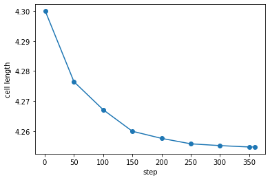
We can also explicitly obtain the final cell length by taking the last element

L0 = float(ops['h[0][0]'][-1]) # store equilib cell length, note: casting as float
print(f"The equilibrium cell length is {L0} Rg")

The equilibrium cell length is 4.25468308 Rg

Field error output files

The field errors throughout the simulation are stored in error.dat. At the moment, this must be loaded into python using np.loadtxt().

%cat error.dat

# step field_error_total dH/mu_plus.l1norm dH/mu_minus.l1normdH/dh.l1norm()
1 1.02646 1.00138 0.0250832 0.0064028
50 0.108101 0.108057 4.40034e-05 0.00668884
100 0.011143 0.0111422 7.87208e-07 0.0030783
150 0.00115259 0.00114892 3.67515e-06 0.00177795
200 0.000118567 0.00011847 9.68855e-08 0.000778028
250 1.31431e-05 1.22159e-05 9.27173e-07 0.000448069
300 1.28438e-06 1.25964e-06 2.47495e-08 0.000195715
350 5.16031e-07 2.82722e-07 2.33309e-07 0.000112648
360 1.15977e-07 1.05155e-07 1.08217e-08 8.54594e-05

Density

The density of each species is output to density.dat. These fields can be loaded and plotted using fieldkit. Fieldkit is included as a submodule in OpenFTS and so if you have set your PYTHONPATH=<path-to-openfts>/build/python correctly, you can import fieldkit without modification

import fieldkit as fk

Now lets load density.dat using fieldkit and plot it

density_fields = fk.read_from_file('density.dat')
fk.plot(density_fields)

Note: not plotting imaginary part of field 0
Note: not plotting imaginary part of field 1

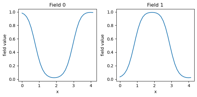
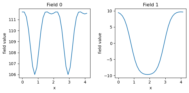
Note that “Field 0” is the density of species A and “Field 1” is the density of species B. As desired, we have obtained the lamellar phase. We can also plot fields.dat (which contains the exchange fields \(w_+\) and \(w_-\), respectively:

exchange_fields = fk.read_from_file('fields.dat')
fk.plot(exchange_fields)

Note: not plotting imaginary part of field 0
Note: not plotting imaginary part of field 1

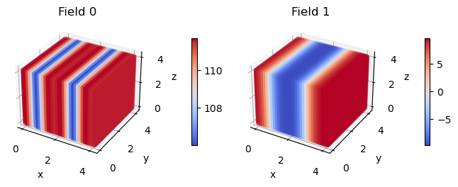
Manipulate fields (1D to 3D)

Now that we have the equilibrium cell length in 1d we can use fieldkit to expand these fields into 3d. This assumes that the fields are homogeneous in the y and z dimensions.

dim_new = 3
npw_new = (32,32) # final cell will be 32x32x32
boxl_new = (L0,L0) # final cell will be cubic
exchange_fields_3d = fk.expand_dimension(exchange_fields, dim_new, npw_new, boxl_new)
fk.plot(exchange_fields_3d)

Note: not plotting imaginary part of field 0
Note: not plotting imaginary part of field 1

Now lets save these fields to a file named ‘exchange_fields_3d.in’

filename = 'exchange_fields_3d.in'
fk.write_to_file(filename,exchange_fields_3d)

Writting 2 fields to exchange_fields_3d.in

3D Complex Langevin

Now we would like to setup a 3d complex Langevin (FTS-CL) simulation. To keep things simple we will create a brand new OpenFTS object (eventually it might be possible to modify the previous OpenFTS object in place. The lines below are generally the same as the example above where changes are noted in the comments.

# create an OpenFTS object
fts = openfts.OpenFTS()

# initialize the cell
# CHANGES FOR CL: now 3d and using L0 for cell length, specifying tilt_factors
fts.cell(cell_scale=L0,cell_lengths=[1,1,1],tilt_factors=[0,0,0],dimension=3,length_unit='Rg')

# initialize the fields
# CHANGES FOR CL: now 32x32x32
fts.field_layout(npw=[32,32,32],random_seed=1)

# initialize the driver (including the field updater and variable cell)
# CHANGES FOR CL: smaller timestep, no stop_tolerance, type="ComplexLangevin",
#                 reduce number of timesteps, no variable cell
#                 add blocksize
fts.driver(dt=0.1,nsteps=1000,output_freq=50,block_size=200, type='ComplexLangevin')
fts.field_updater(type='EMPEC',update_order='simultaneous',adaptive_timestep=False,lambdas=[1.0, 1.0])

# number of beads in chain
N = 50

# Create the model with chiN=20 and BC=100
# CHANGES FOR CL: need to specify C
fts.model(type='MeltChiAB', Nref=N,bref=1.0,chiN=20.,inverse_BC=0.01, C=5)

# initialize the model fields
# CHANGES FOR CL: initialize from our newly created file
fts.init_fields_from_file(filename, field_type='exchange')



# create a molecule, here a diblock consisting of N beads with fA=0.5
fts.add_molecule(type='PolymerLinear',chain_type='discrete',
                 nbeads=N,nblocks=2,block_fractions=[0.5, 0.5],block_species=['A', 'B'],
                 volume_frac=1.0)

# Set the operators we seek to output
# CHANGES FOR CL: add the chemical potential, pressure, and DensitySpecies operator,
#                 remove cell stress operator
fts.add_operator(averaging_type='none',type='Hamiltonian')
fts.add_operator(averaging_type='none',type='Pressure')
fts.add_operator(averaging_type='none',type='ChemicalPotential')
fts.add_operator(averaging_type='block',type='DensitySpecies')

# Use the default names of output files
fts.output_default()

# Use two species types A and B, each with a smearing length of 0.15 Rg
fts.add_species(label='A',stat_segment_length=1.0, smearing_length=0.15)
fts.add_species(label='B',stat_segment_length=1.0, smearing_length=0.15)

Here’s a summary of the changes from the original SCFT input:

1. The cell and npw were changed to 3 dimensions

2. The exchange fields are initialized using exchange_fields_3d.dat

3. We have updated the driver to be “ComplexLangevin”. We are also no longer using variable cell.

4. We have added the “ChemicalPotential”, “Pressure” and “DensitySpecies” operators

Now we’re ready to run. A few notes:

* This could take a few minutes since we're now in 3d.
* This will overwrite the files created by our earlier SCFT run

fts.run()

============================================================
                          OpenFTS

OpenFTS version: heads/develop 1e8cdcf DIRTY
FieldLib version: heads/master e7d9bf6 CLEAN
Execution device: [CPU]
FieldLib precision: double
=============================================================

Initialize Cell
  * dim = 3
  * length unit = Rg
  * cell_lengths = [4.254683 4.254683 4.254683 ]
  * tilt_factors = [0.000000 0.000000 0.000000 ]
  * cell_tensor:
4.25 0.00 0.00
0.00 4.25 0.00
0.00 0.00 4.25
Initialize FieldLayout
  * npw = [32 32 32 ]
  * random_seed = 1
Initialize Species
  * label = A
  * stat_segment_length = 1.000000
  * smearing_length = 0.150000
  * charge = 0.000000
Initialize Species
  * label = B
  * stat_segment_length = 1.000000
  * smearing_length = 0.150000
  * charge = 0.000000
Initialize ModelMeltChiAB
  * bref = 1.00
  * Nref = 50.00
  * chiN = 20.00
  * C = 5.00
  * compressibility_type = exclvolume
  * inverse_BC = 0.01
  * initfields = yes
    *  reading 'exchange' fields from file 'exchange_fields_3d.in'
Initialize MoleculePolymerLinear
  * volume_frac = 1.00
  * chain_type = discrete
  * Linear polymer has single chain:
    - type = discrete
    - nbeads = 50
    - discrete_type = Gaussian
    - sequence_type = blocks
    - nblocks = 2
    - block_fractions =  0.500000 0.500000
    - block_species =  A B
    - monomer_sequence (compact) =  A_25 B_25
    - monomer_sequence (long) = AAAAAAAAAAAAAAAAAAAAAAAAABBBBBBBBBBBBBBBBBBBBBBBBB
Initialize DriverSCFTCL
  * is_complex_langevin = true
  * dt = 0.100000
  * output_freq = 50
  * block_size = 200
  * field_updater = EMPEC
    - adaptive_timestep = false
    - predictor_corrector = true
    - update_order = simultaneous
    - lambdas = 1.000000 1.000000
Calculating Operators:
  * OperatorChemicalPotential
    - type = scalar
    - averaging_type = none
    - save_history = true
    - incl_ideal_gas = 1
  * OperatorDensitySpecies
    - type = field
    - averaging_type = block
    - save_history = false
  * OperatorHamiltonian
    - type = scalar
    - averaging_type = none
    - save_history = true
  * OperatorPressure
    - type = scalar
    - averaging_type = none
    - save_history = true
    - incl_ideal_gas = true
Output to files:
  * scalar_operators  -> "operators.dat"
  * species_densities -> "density.dat"
                      ->  save_history = false
  * exchange_fields   -> "fields.dat"
                      ->  save_history = false
  * field_errors      -> "error.dat"

Running DriverSCFTCL
  * nsteps = 1000

Starting Run.
Step:      1  H: 2.940286e+02 +9.185379e-03i  Q: 7.640e-47 +1.807e-50i  TPS:   5.64
Step:     50  H: 5.633244e+02 -2.866321e-02i  Q: 3.841e-47 -4.588e-48i  TPS:   8.87
Step:    100  H: 6.135196e+02 +3.893494e-02i  Q: 3.376e-47 +7.363e-48i  TPS:   8.82
Step:    150  H: 6.474557e+02 -1.672611e-01i  Q: 2.944e-47 +6.961e-48i  TPS:   8.75
Step:    200  H: 6.639935e+02 -1.320669e-01i  Q: 1.749e-47 -1.602e-48i  TPS:   8.81
Step:    250  H: 6.716861e+02 -2.483724e-02i  Q: 2.761e-47 +6.825e-49i  TPS:   8.79
Step:    300  H: 6.841572e+02 -1.699686e-01i  Q: 3.118e-47 +8.656e-48i  TPS:   8.75
Step:    350  H: 6.841998e+02 +1.737971e-01i  Q: 1.916e-47 +1.046e-47i  TPS:   8.74
Step:    400  H: 6.903463e+02 +3.471909e-01i  Q: 1.815e-47 +1.801e-47i  TPS:   8.77
Step:    450  H: 6.902785e+02 +9.104579e-02i  Q: 1.738e-47 +1.187e-47i  TPS:   8.76
Step:    500  H: 6.918223e+02 -1.836392e-01i  Q: 2.618e-47 -9.193e-48i  TPS:   8.82
Step:    550  H: 6.930252e+02 -7.521176e-02i  Q: 3.612e-47 -5.283e-48i  TPS:   8.83
Step:    600  H: 6.952256e+02 -2.507921e-01i  Q: 2.736e-47 -7.241e-49i  TPS:   8.90
Step:    650  H: 6.939332e+02 +2.114412e-01i  Q: 2.420e-47 +1.934e-48i  TPS:   8.82
Step:    700  H: 6.930407e+02 -6.773803e-02i  Q: 2.064e-47 -4.000e-49i  TPS:   8.85
Step:    750  H: 6.926380e+02 -3.546703e-01i  Q: 2.430e-47 -2.490e-48i  TPS:   8.81
Step:    800  H: 6.956517e+02 +4.275557e-01i  Q: 3.037e-47 -1.000e-47i  TPS:   8.88
Step:    850  H: 6.994019e+02 -2.348493e-01i  Q: 2.385e-47 -8.696e-48i  TPS:   8.83
Step:    900  H: 6.981663e+02 -2.658321e-02i  Q: 1.912e-47 -3.428e-49i  TPS:   8.79
Step:    950  H: 6.977495e+02 -2.219257e-01i  Q: 2.657e-47 +3.533e-48i  TPS:   8.82
Step:   1000  H: 6.965320e+02 -6.803616e-02i  Q: 2.431e-47 +4.843e-48i  TPS:   8.78
Run reached specified number of steps
Run completed in 113.99 seconds (8.77 steps / sec).

Now lets plot the operators that were generated

# Load operators
ops = openfts.get_scalar_operators(fts, mode='timeseries')

# Plot them
fig = plt.figure(figsize=(2*3.33,3.33),dpi=100)
axes = fig.subplots(3,2,sharex=True)

for i,ikey in enumerate(['H', 'mu_0','P']):
    for j,jkey in enumerate(['.real','.imag']):
        if i == 2:
            axes[i][j].set_xlabel('step')
        axes[i][j].set_ylabel(ikey + jkey)
        axes[i][j].plot(ops['step'],ops[ikey+jkey],marker='o')
plt.tight_layout()
plt.show()

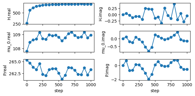
As anticipated in CL, there is a brief ‘warm-up’ before these operators reach their equilibrium values and the imaginary component of these operators are fluctuating around zero. This runtime was quite short to keep this example managable. In practice, you will have to run much longer to get good statistics.

We can also plot the density in density.dat.

density_fields = fk.read_from_file('density.dat')
fk.plot(density_fields)

Note: not plotting imaginary part of field 0
Note: not plotting imaginary part of field 1

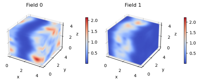
These densities are quite noisy! This is because density.dat contains the * instantaneous density. This can have a large imaginary component and can have densities outside of the expected range of 0-1. In CL, the instantaneous density does not have physical meaning.

Instead, you should look at the average density. Averaging can be performed internally from within OpenFTS by setting averaging_type='block' inside of an operator. In fact, we did this when setting up you CL inputs above (though you may have missed it):

fts.add_operator(averaging_type='block',type='DensitySpecies')

This operator creates a new output file called opDensitySpecies.dat which contains the instantaneous density averaged over the block_size specified in driver. When we plot these densities, the density profile is much cleaner.

density_fields = fk.read_from_file('opDensitySpecies.dat')
fk.plot(density_fields)

Note: not plotting imaginary part of field 0
Note: not plotting imaginary part of field 1

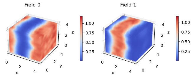
The big takeaway is that you should always look at averaged operators in CL simulations. This averaging can be done internally within OpenFTS (as we just saw for the density) or as a postprocessing step.

Particle-based simulations

As a final step of this example workflow, we will now convert our OpenFTS inputs into an identical particle-based simulation. To get our bearings, lets first look at the files in our directory

%ls

density.dat             fields.dat         opDensitySpecies.dat  STATUS
error.dat               frame_0000000.png  operators.dat
example_workflow.ipynb  fresnel.log        polymer.gsd
exchange_fields_3d.in   from-fresnel.png   polymer.json

Creating all of the inputs for a particle-based simulation only takes a single line. Here we will demonstrate this with HOOMD, but you can also generate inputs for LAMMPS.

fts.map_to_particle(simulation_type='hoomd',file_prefix='polymer')

Generated Particle Configuration:
  * natoms =  19250
  * nmolecules = 385
  * rho0 =  10.71
  * C_actual =  5.00
Writing HOOMD input files:
  * gsdfile = polymer.gsd
  * jsonfile = polymer.json

This has generated two new files polymer.json and polymer.gsd. polymer.json contains the information needed to run a HOOMD simulation. These include bonded and non-bonded interaction parameters as well as information about the cell.

%cat polymer.json

{
  "bond": {
    "kbond": [
      3.0,
      3.0,
      3.0
    ],
    "r0": [
      0.0,
      0.0,
      0.0
    ]
  },
  "config": {
    "cell": [
      12.158769657128664,
      12.158769657128664,
      12.158769657128664,
      0.0,
      0.0,
      0.0
    ],
    "natoms": 19250,
    "nmolecules": 385,
    "nmolecules_per_type": [
      385
    ],
    "rho0": 10.709318646510402
  },
  "pair": {
    "gauss_A_0": -0.05321099914819749,
    "gauss_A_AB": -0.06385319897783698,
    "gauss_B": 1.3605442176870748,
    "gauss_eps_0": 0.05321099914819749,
    "gauss_eps_AB": 0.06385319897783698,
    "gauss_sig": 0.6062177826491071,
    "rcut": 2.727980021920982
  },
  "species": {
    "labels": [
      "A",
      "B"
    ],
    "nspecies": 2
  }
}

polymer.gsd contains the initial coordinates of all atoms in the system and the topology of the molecules (i.e. which atoms are bonded together). If you have fresnel installed, you can directly visualize this file using the script OpenFTS/python/tools/render-with-fresnel.py. Alternatively you can use VMD, Ovito or your visualization tool of choice. An example command is:

<path>/render-with-fresnel.py -i polymer.gsd --height 20 --production

This will generate frame_0000000.png. Here’s what it looks like:

from IPython.display import Image
Image(filename='frame_0000000.png')

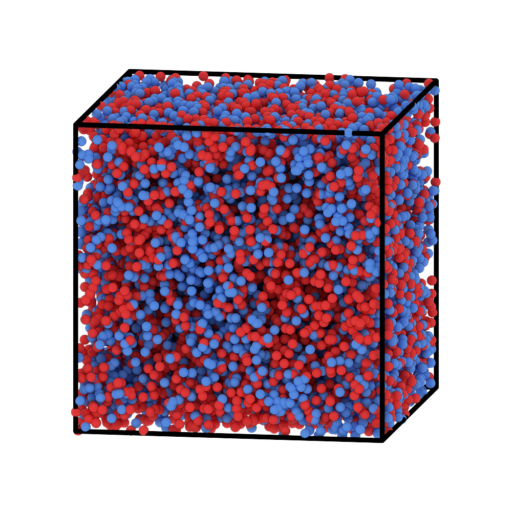
You’re now ready to run a simulation. A sample HOOMD script can be found at OpenFTS/examples/particlemap/ModelMeltChiAB/via-map-to-particle/hoomd3/run-hoomd3.py.

That it! You can now start running molecular dynamics simulations with the exact same model used in OpenFTS. Neat.