Mapping from fields to particles

OpenFTS is primarily a field-theoretic simulation code, but it also makes it easy to setup and run equivalent particle-based simulations using LAMMPS and HOOMD. There are many reasons why you might want to do this:

1. You want to know what the individual chains are doing (FTS doesn’t have this information)

2. You want information about the system’s dynamics (FTS doesn’t have dynamics)

3. You want to look at fluctuations, but dont want to run FTS (CL is sometimes finicky)

4. You are having issues with FTS (CL is not perfect)

5. You want to confirm that OpenFTS is right by double-checking with a particle simulation (bugs do exist!)

Because running equivalent particle-based simulations is so useful, OpenFTS makes running particle-based simulations very easy. In fact, in most cases you can initialize a particle-based simulation by only adding a single line to your existing OpenFTS input file. All those annoying unit conversions from FTS units (lengths in \(R_g\), concentrations in \(C = \rho_0 R_g^3 / N\), etc) are taken care of for you under the hood.

Sound interesting? Lets get started.

For this example, we’ll look at a two component mixture consisting of a AB diblock copolymer in a B solvent. We will choose \(f_A = 0.28\) and polymer volume fraction \(\phi = 0.3\) so that this system forms micelles.

To run this tutorial yourself, you will need:

1. A LAMMPS executable lmp_mpi in your PATH env variable that has been compiled with the fix_density_field plug-in.

2. Both openfts and fresnel in your PYTHONPATH env variable.

Setup and initial SCFT

Our first step when examining this system will be to run SCFT. SCFT runs very fast and this will let us quicky see if these parameters yield micelles as expected.

import openfts

# create an OpenFTS object
fts = openfts.OpenFTS()

# initialize 3d cell
fts.cell(cell_scale=4.0,cell_lengths=[1,1,1],tilt_factors=[0,0,0],dimension=3,length_unit='Rg')
fts.field_layout(npw=[16,16,16],random_seed=1975)

# run SCFT
fts.driver(dt=5.0,nsteps=4000,output_freq=100,type='SCFT',stop_tolerance=1e-4)
fts.field_updater(type='EMPEC',update_order='simultaneous',adaptive_timestep=False,lambdas=[1.0, 1.0])

# number of beads in chain
N = 50

# Create the model with chiN=20 and BC=100, C=5
# note: C is ignored by SCFT but will be used when we initialize the particle simulations
fts.model(type='MeltChiAB', Nref=N,bref=1.0,chiN=100,inverse_BC=0.01,C=5)


# initialize the model fields
fts.init_model_field(fieldname='mu_plus',type='random',mean=0.0,stdev=1.0)
fts.init_model_field(fieldname='mu_minus',type='random',mean=0.0,stdev=1.0)


phi = 0.30 # polymer volume fraction

# diblock
fts.add_molecule(type='PolymerLinear',chain_type='discrete',
                 nbeads=N,nblocks=2,block_fractions=[0.28, 0.72],block_species=['A', 'B'],
                 volume_frac=phi)
# create a solvent molecule, (i.e. a N=1 polymer)
fts.add_molecule(type='PolymerLinear',chain_type='discrete',
                 nbeads=1,nblocks=1,block_fractions=[1.0],block_species=['B'],
                 volume_frac=1-phi)

# Set the operators we seek to output
fts.add_operator(type='Hamiltonian', averaging_type='none')

# Use the default names of output files
fts.output_default()

# Use two species types A and B, each with a smearing length of 0.15 Rg
fts.add_species(label='A',stat_segment_length=1.0, smearing_length=0.15)
fts.add_species(label='B',stat_segment_length=1.0, smearing_length=0.15)

Now that our simulation is setup lets run SCFT:

fts.run()

============================================================
                          OpenFTS

OpenFTS version: heads/develop 0c946a7 DIRTY
FieldLib version: heads/master 9f8b95c CLEAN
Execution device: [GPU 0] NVIDIA GeForce RTX 2080 Ti (ComputeCapability 7.5)
FieldLib precision: double
=============================================================

Initialize Cell
  * dim = 3
  * length unit = Rg
  * cell_lengths = [4.000000 4.000000 4.000000 ]
  * tilt_factors = [0.000000 0.000000 0.000000 ]
  * cell_tensor:
4 0 0
0 4 0
0 0 4
Initialize FieldLayout
  * npw = [16 16 16 ]
  * random_seed = 1975
Initialize Species
  * label = A
  * stat_segment_length = 1.000000
  * smearing_length = 0.150000
  * charge = 0.000000
Initialize Species
  * label = B
  * stat_segment_length = 1.000000
  * smearing_length = 0.150000
  * charge = 0.000000
Initialize ModelMeltChiAB
  * bref = 1
  * Nref = 50
  * chiN = 100
  * C = 5
  * compressibility_type = exclvolume
  * inverse_BC = 0.01
  * initfields = yes
Initialize MoleculePolymerLinear
  * volume_frac = 0.3
  * chain_type = discrete
  * Linear polymer has single chain:
    - type = discrete
    - nbeads = 50
    - discrete_type = Gaussian
    - sequence_type = blocks
    - nblocks = 2
    - block_fractions =  0.280000 0.720000
    - block_species =  A B
    - monomer_sequence (compact) =  A_14 B_36
    - monomer_sequence (long) = AAAAAAAAAAAAAAABBBBBBBBBBBBBBBBBBBBBBBBBBBBBBBBBBB
Initialize MoleculePolymerLinear
  * volume_frac = 0.7
  * chain_type = discrete
  * Linear polymer has single chain:
    - type = discrete
    - nbeads = 1
    - discrete_type = Gaussian
    - sequence_type = blocks
    - nblocks = 1
    - block_fractions =  1.000000
    - block_species =  B
    - monomer_sequence (compact) =  B_1
    - monomer_sequence (long) = B
Initialize DriverSCFTCL
  * is_complex_langevin = false
  * dt = 5.000000
  * output_freq = 100
  * block_size = 100
  * field_updater = EMPEC
    - predictor_corrector = true
    - update_order = simultaneous
    - lambdas = 1.000000 1.000000     - adaptive_timestep = false

  * field_stop_tolerance = 0.0001
Calculating Operators:
  * OperatorHamiltonian
    - type = scalar
    - averaging_type = none
    - save_history = true
Output to files:
  * scalar_operators  -> "operators.dat"
  * species_densities -> "density.dat"
                      ->  save_history = false
  * exchange_fields   -> "fields.dat"
                      ->  save_history = false
  * field_errors      -> "error.dat"

Running DriverSCFTCL
  * nsteps = 4000

Starting Run.
Step:      1  H: 1.702577e+00 -5.166810e-20i  Q: 3.590e-02 +2.687e-21i  FieldErr: 1.82e+00  TPS:  52.93
Step:    100  H: 5.580338e+01 -1.678100e-16i  Q: 9.300e-50 +4.199e-65i  FieldErr: 4.13e-02  TPS:  97.80
Step:    200  H: 5.589665e+01 +1.520165e-16i  Q: 5.269e-52 -1.396e-67i  FieldErr: 1.70e-03  TPS: 100.04
SCFT converged in 295 steps to tolerance: 0.00 (fields)
* H = 55.8968 -1.49687e-16i
Run completed in 3.00 seconds (97.85 steps / sec).

Now lets visualize the densities using fieldkit. We can first visualize the species densities. In this case Field 0 is species A and Field 1 is species B.

import fieldkit as fk
density_fields = fk.read_from_file('density.dat')
fk.plot(density_fields)

Note: not plotting imaginary part of field 0
Note: not plotting imaginary part of field 1

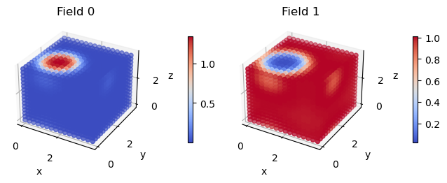
As expected, we got a micelle. Cool!

Mapping to LAMMPS

Now lets run a particle based simulation that corresponds exactly to the SCFT simulation we just ran. OpenFTS makes it easy to setup simulations in both LAMMPS and HOOMD.

In order to generate all of the inputs needed for a LAMMPS simulation, you only need to add a single line to your existing OpenFTS python input file:

fts.map_to_particle(simulation_type='lammps',file_prefix='polymer')

Generated Particle Configuration:
  * natoms =  16000
  * nmolecules = 11296
  * rho0 =  10.71
  * C_actual =  5.00
Writing LAMMPS input files:
  * datafile = polymer.data
  * coefffile = polymer.coeff
  * xyzfile = polymer.xyz
  * psffile = polymer.psf

OpenFTS give you some general information about the particle-based simulation you just generated (number of atoms, number of molecules, density, etc).

More importantly, it generates an input configuration, topology, and force-field parameters that are needed to run LAMMPS. Specifically, the files generated by OpenFTS are as follows:

• data file - particle positions, bonds and box information to be read using the LAMMPS read_data command.

• coeff file - file specifying the pair and bond types/styles to use in LAMMPS. This file can be conveniently read into a LAMMPS input file using the LAMMPS include command.

• xyz file - xyz coordinates of particles. Useful for quickly vizualizing initial configuration

• psf file - contains topology information of configuration. Useful for visualization or for compatability with tools like mdtraj.

• in.lammps - this is a file that you need to actually run lammps

Perhaps you can tell that there’s alot of heavy lifting that is going on behind the scenes here. OpenFTS only knows about the FTS parameters (i.e. \(\chi N\), \(C\), all lengths in \(R_g\), etc) but it generates input files in units that LAMMPS can understand (i.e. lengths, energies in Lennard-Jones units). It also converts the abstract language of OpenFTS “molecules” (i.e. block fraction = 0.28, volume_fraction = 0.3) and writes actual particles that are bonded together at the right density and at a consistent box size.

Taken together, these LAMMPS input files will run exactly the same model as implemented in OpenFTS. We wont do it in this tutorial, but you can test this: run complex Langevin and LAMMPS and you will get exactly the same pressure. But I digress..

Finally, lets take a look at in.lammps

!cat in.lammps

# LAMMPS input script for use with OpenFTS generated input files

# Random number seed for orientation
variable random equal 12345
variable T equal 1
variable freq equal 100
variable freqhalf equal ${freq}/2
variable isRestart equal 0

units           lj
atom_style      bond
dimension 3

# Read in the configuration
if "${isRestart} == 0" then &
  "read_data polymer.data" &
else &
  "read_restart restart.*"

mass * 1.0
velocity all create ${T} ${random}

include polymer.coeff

neighbor        1.5 bin
neigh_modify    every 20 delay 0 check yes  page 5100000 one 500000
timestep 0.005

fix 1 all langevin ${T} ${T} 0.5 ${random}
###fix rhobias all density_field 10.0 200 200 4 ${freq} 2 density.dat 1 0 rhoA.dat density.dat 2 1 rhoB.dat
fix 3 all nve

dump    1 all atom ${freq} dump.lammpstrj
dump_modify 1 scale no

if "${isRestart} == 1" then &
  "dump_modify 1 append yes"

thermo ${freq}
###thermo_style custom step ebond epair pe temp press f_rhobias

restart ${freqhalf} restart.0 restart.1
run     1000

This input file is pretty simple if you’re already familiar with LAMMPS. A very nifty feature of this input file it is very generic: no configuration or model specific parameters are written in this input file. Instead, all of this information is contained in polymer.data and polymer.coeff which are then read by this file. Essentially this means that in.lammps only contains instructions on how to run LAMMPS, while polymer.data and polymer.coeff specify what system should be run. This means if you want to change your simulation conditions (i.e. change \(\phi\) or add a 3rd component to the system), in.lammps will remain unchanged and the only place you’ll need to make changes is in the OpenFTS input files (which ultimately write polymer.data and polymer.coeff).

Now that we’ve explained in.lammps, we can now run it using LAMMPS. This assumes that the LAMMPS executable is in your PATH env variable. Note that this step should take about a minute to run.

!mpirun -np 4 lmp_mpi -i in.lammps

Ignoring PCI device with non-16bit domain.
Pass --enable-32bits-pci-domain to configure to support such devices
(warning: it would break the library ABI, don't enable unless really needed).
LAMMPS (29 Sep 2021)
Reading data file ...
  orthogonal box = (-5.7154800 -5.7154800 -5.7154800) to (5.7154800 5.7154800 5.7154800)
  1 by 2 by 2 MPI processor grid
  reading atoms ...
  16000 atoms
  scanning bonds ...
  1 = max bonds/atom
  reading bonds ...
  4704 bonds
Finding 1-2 1-3 1-4 neighbors ...
  special bond factors lj:    0        0        0
  special bond factors coul:  0        0        0
     2 = max # of 1-2 neighbors
     2 = max # of 1-3 neighbors
     4 = max # of 1-4 neighbors
     6 = max # of special neighbors
  special bonds CPU = 0.002 seconds
  read_data CPU = 0.046 seconds
Finding 1-2 1-3 1-4 neighbors ...
  special bond factors lj:    1        1        1
  special bond factors coul:  1        1        1
     2 = max # of 1-2 neighbors
     6 = max # of special neighbors
  special bonds CPU = 0.001 seconds
Neighbor list info ...
  update every 20 steps, delay 0 steps, check yes
  max neighbors/atom: 500000, page size: 5100000
  master list distance cutoff = 4.22798
  ghost atom cutoff = 4.22798
  binsize = 2.11399, bins = 6 6 6
  1 neighbor lists, perpetual/occasional/extra = 1 0 0
  (1) pair gauss, perpetual
      attributes: half, newton on
      pair build: half/bin/newton
      stencil: half/bin/3d
      bin: standard
Setting up Verlet run ...
  Unit style    : lj
  Current step  : 0
  Time step     : 0.005
WARNING: Inconsistent image flags (../domain.cpp:814)
Per MPI rank memory allocation (min/avg/max) = 53.93 | 53.94 | 53.95 Mbytes
Step Temp E_pair E_mol TotEng Press
       0            1    1.1862272   0.44232679    3.1284603    20.169278
     100    1.0092376    1.1643711   0.44431089    3.1224439    20.140285
     200    1.0169425    1.1507128    0.4530603    3.1290916     20.05718
     300    1.0104167    1.1461058   0.45499263    3.1166288    19.940364
     400    1.0108423    1.1449761   0.44730148    3.1084463    19.973688
     500    1.0114452    1.1442145   0.44580823    3.1070958    19.991495
     600    0.9996872    1.1450925   0.43939529    3.0839248    19.913484
     700     1.004258    1.1432745   0.44000005    3.0895675    19.957904
     800    1.0021221    1.1421812   0.44044096    3.0857113    19.923128
     900    1.0000447    1.1415486    0.4398611    3.0813829     19.89254
    1000    1.0031849    1.1421794   0.44454282    3.0914054    19.891883
Loop time of 67.0097 on 4 procs for 1000 steps with 16000 atoms

Performance: 6446.823 tau/day, 14.923 timesteps/s
99.6% CPU use with 4 MPI tasks x no OpenMP threads

MPI task timing breakdown:
Section |  min time  |  avg time  |  max time  |%varavg| %total
---------------------------------------------------------------
Pair    | 51.579     | 55.496     | 59.844     |  45.2 | 82.82
Bond    | 0.016208   | 0.019856   | 0.022841   |   2.0 |  0.03
Neigh   | 6.056      | 6.0563     | 6.0566     |   0.0 |  9.04
Comm    | 0.83724    | 5.182      | 9.0989     | 147.9 |  7.73
Output  | 0.052294   | 0.052447   | 0.052663   |   0.1 |  0.08
Modify  | 0.15347    | 0.15718    | 0.15966    |   0.6 |  0.23
Other   |            | 0.0459     |            |       |  0.07

Nlocal:        4000.00 ave        4104 max        3946 min
Histogram: 2 0 1 0 0 0 0 0 0 1
Nghost:        38547.0 ave       38904 max       38172 min
Histogram: 1 0 0 1 0 0 1 0 0 1
Neighs:    6.78316e+06 ave  7.1643e+06 max 6.47538e+06 min
Histogram: 2 0 0 0 0 0 0 1 0 1

Total # of neighbors = 27132646
Ave neighs/atom = 1695.7904
Ave special neighs/atom = 0.58800000
Neighbor list builds = 39
Dangerous builds = 0
Total wall time: 0:01:07

This generates a trajectory in dump.lammpstrj. We can vizualize it by using some utility scripts included with OpenFTS. We wont go into the details of these scripts here – the jist is that they generate png snapshots along the trajectory.

You can also visualize the trajectory with VMD: vmd dump.lammpstrj polymer.psf

!../../../../python/tools/lammpstrj_to_gsd.py -lmp dump.lammpstrj -psf polymer.psf -r 0 -1 -o from-lammps.gsd
!../../../../python/tools/render-with-fresnel.py -i from-lammps.gsd --start 0 --stop 10 --height 20 --step 10 --cameraup z --camerapos 30 -50 60 --frameprefix nobias

Converting frames 0 to 10 w/ step None of dump.lammpstrj (topology polymer.psf) to from-lammps.gsd
Rendering 'from-lammps.gsd': frames 0 to 10 every 10 (of 11 total).
<fresnel.Device: Enabled OptiX devices:
 [0]: NVIDIA GeForce RTX 2080 Ti   68 SM_7.5 @ 1.65 GHz,  5602 MiB DRAM
>
Rendered nobias_0000000.png in 0.24 seconds, Time elapsed = 0.24 s, ETA = 0.24 s
Rendered nobias_0000010.png in 0.15 seconds, Time elapsed = 0.39 s, ETA = 0.00 s

After this short LAMMPS run (1000 steps), the initial and final configuration of the system is:

Initial Frame	Final Frame

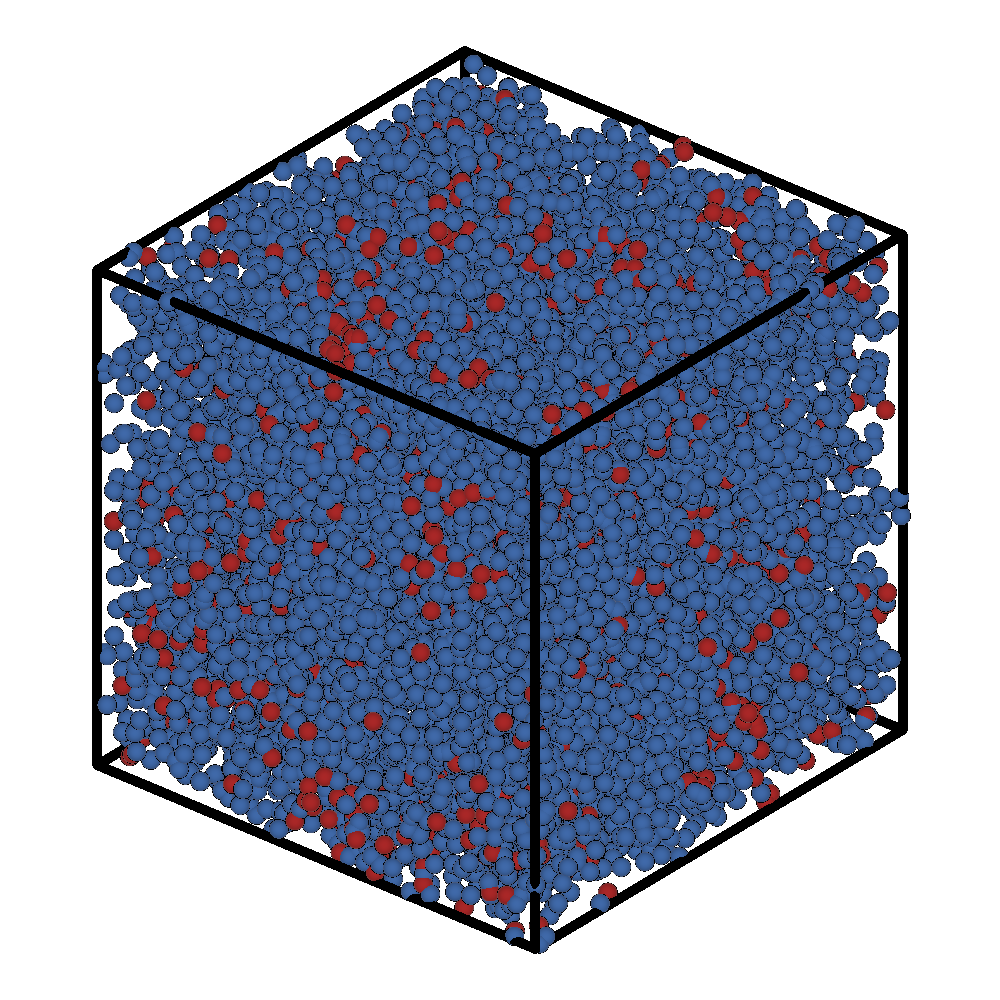
If we ran LAMMPS for a very long time we should see the formation of a micelle.

LAMMPS with a bias

Since we already used SCFT to equilibrate the system, a smarter way to equilibrate our MD system is to In order to more quickly equilibrate this system we will use a custom LAMMPS fix called fix_density_field. Detailed documentation on fix_density_field is given elsewhere and we’ll mostly focusing on using this fix here.

As it turns out, the modifications needed to use this fix are already included in the in.lammps file we used above (but were commented out). Each of these lines contain the rhobias string and so we can uncomment them using sed and save them into a new file in.lammps-bias:

!sed -e '/rhobias/s/###//g' < in.lammps >in.lammps-bias

Lets take a look at the relevant lines using grep:

!grep -n rhobias in.lammps-bias

30:fix rhobias all density_field 10.0 200 200 4 ${freq} 2 density.dat 1 0 rhoA.dat density.dat 2 1 rhoB.dat
40:thermo_style custom step ebond epair pe temp press f_rhobias

Lets discuss these two lines one by one:

1. The first line (line 30) is where most of the magic happens. This is where we are adding new fix in order to push it towards some density field of interest. Here we will bias it towards the density fields in density.dat that we obtained at the start of this tutorial using SCFT. The other arguments tell this fix:

   • how strong should the bias be

   • when should the bias be applied

   • where to write the instantaneous MD density fields (rhoA.dat and rhoB.dat)

   • which LAMMPS species indicies correspond to which columns of density.dat

   • See the fix_density_field documentation for more information.

2. The second line (line 40) adds this fix to the thermo output. This will help us understand if the bias is working correctly.

We’re now ready to run LAMMPS using this bias potential (this should take about 5 minutes to run):

!mpirun -np 4 lmp_mpi -i in.lammps-bias

Ignoring PCI device with non-16bit domain.
Pass --enable-32bits-pci-domain to configure to support such devices
(warning: it would break the library ABI, don't enable unless really needed).
LAMMPS (29 Sep 2021)
Reading data file ...
  orthogonal box = (-5.7154800 -5.7154800 -5.7154800) to (5.7154800 5.7154800 5.7154800)
  1 by 2 by 2 MPI processor grid
  reading atoms ...
  16000 atoms
  scanning bonds ...
  1 = max bonds/atom
  reading bonds ...
  4704 bonds
Finding 1-2 1-3 1-4 neighbors ...
  special bond factors lj:    0        0        0
  special bond factors coul:  0        0        0
     2 = max # of 1-2 neighbors
     2 = max # of 1-3 neighbors
     4 = max # of 1-4 neighbors
     6 = max # of special neighbors
  special bonds CPU = 0.001 seconds
  read_data CPU = 0.043 seconds
Finding 1-2 1-3 1-4 neighbors ...
  special bond factors lj:    1        1        1
  special bond factors coul:  1        1        1
     2 = max # of 1-2 neighbors
     6 = max # of special neighbors
  special bonds CPU = 0.001 seconds
fix density_field info ...
  k_bias_in = 10, nsteps_on = 200, nsteps_period = 200
  assignment_function_order = 4
  output_frequency = 100
  nbiasfields = 2
  target_density_filename = density.dat, species_to_bias = 1, field_index_to_read = 0, output_filename = rhoA.dat
  target_density_filename = density.dat, species_to_bias = 2, field_index_to_read = 1, output_filename = rhoB.dat
  FIX_DENSITY_DEBUG_FLAG = 0 (this is hardoded, must recompile to change)
Setting up fix_density_field for run ...
  avg_particle_per_grid_pt (natoms*P/npw)= 15.625
  natoms = 16000 npw = 4096 P = 4
Neighbor list info ...
  update every 20 steps, delay 0 steps, check yes
  max neighbors/atom: 500000, page size: 5100000
  master list distance cutoff = 4.22798
  ghost atom cutoff = 4.22798
  binsize = 2.11399, bins = 6 6 6
  1 neighbor lists, perpetual/occasional/extra = 1 0 0
  (1) pair gauss, perpetual
      attributes: half, newton on
      pair build: half/bin/newton
      stencil: half/bin/3d
      bin: standard
Setting up Verlet run ...
  Unit style    : lj
  Current step  : 0
  Time step     : 0.005
WARNING: Inconsistent image flags (../domain.cpp:814)
Per MPI rank memory allocation (min/avg/max) = 53.93 | 53.94 | 53.95 Mbytes
Step E_bond E_pair PotEng Temp Press f_rhobias
       0   0.44232679    1.1862272     1.628554            1    20.169278      1.04108
     100   0.46478398    1.1538908    1.6186748    1.0465389    20.370056   0.75663608
     200   0.46612224      1.15698    1.6231023    1.0183765    20.089531   0.65059938
     300   0.46209075    1.1566747    1.6187655    1.0128058    20.059453   0.59281559
     400   0.45679041    1.1519493    1.6087397    1.0135055    20.058282   0.56084162
     500   0.46594245    1.1466955    1.6126379   0.99434679    19.735269   0.53972145
     600   0.46445412    1.1428158    1.6072699    1.0043035    19.810852   0.52364472
     700   0.46449749    1.1380472    1.6025446    1.0055613    19.788571   0.50186938
     800   0.46393275    1.1338887    1.5978215    1.0055995    19.750953   0.48964143
     900   0.45948487    1.1319394    1.5914243   0.99886535    19.683124   0.47828551
    1000   0.45878188    1.1279468    1.5867287    1.0014817    19.682787   0.46230795
Loop time of 302.745 on 4 procs for 1000 steps with 16000 atoms

Performance: 1426.944 tau/day, 3.303 timesteps/s
99.9% CPU use with 4 MPI tasks x no OpenMP threads

MPI task timing breakdown:
Section |  min time  |  avg time  |  max time  |%varavg| %total
---------------------------------------------------------------
Pair    | 50.991     | 55.788     | 60.773     |  52.3 | 18.43
Bond    | 0.016603   | 0.020378   | 0.02321    |   1.9 |  0.01
Neigh   | 6.1726     | 6.1729     | 6.1732     |   0.0 |  2.04
Comm    | 3.5265     | 9.1434     | 15.033     | 140.5 |  3.02
Output  | 0.098062   | 0.2032     | 0.28873    |  15.2 |  0.07
Modify  | 230.01     | 231.2      | 232.43     |   6.4 | 76.37
Other   |            | 0.2162     |            |       |  0.07

Nlocal:        4000.00 ave        4114 max        3772 min
Histogram: 1 0 0 0 0 0 0 1 1 1
Nghost:        38951.5 ave       39760 max       38213 min
Histogram: 1 0 0 0 2 0 0 0 0 1
Neighs:    6.79534e+06 ave 7.24909e+06 max  6.2192e+06 min
Histogram: 1 0 0 0 1 0 0 0 1 1

Total # of neighbors = 27181369
Ave neighs/atom = 1698.8356
Ave special neighs/atom = 0.58800000
Neighbor list builds = 39
Dangerous builds = 0
Total wall time: 0:05:03

An important piece of the LAMMPS output to keep an eye on is the f_rhobias column in the thermo output. This is the total energy associated with the bias potential and should be going down if fix_density_field is working correctly.

Now that our biased LAMMPS simulation is done we can visualize the first and last frames.

!../../../../python/tools/lammpstrj_to_gsd.py -lmp dump.lammpstrj -psf polymer.psf -r 0 -1 -o from-lammps.gsd
!../../../../python/tools/render-with-fresnel.py -i from-lammps.gsd --start 0 --stop 10 --height 20 --step 10 --cameraup z --camerapos 30 -50 60 --frameprefix bias

Converting frames 0 to 10 w/ step None of dump.lammpstrj (topology polymer.psf) to from-lammps.gsd
Rendering 'from-lammps.gsd': frames 0 to 10 every 10 (of 11 total).
<fresnel.Device: Enabled OptiX devices:
 [0]: NVIDIA GeForce RTX 2080 Ti   68 SM_7.5 @ 1.65 GHz,  5602 MiB DRAM
>
Rendered bias_0000000.png in 0.28 seconds, Time elapsed = 0.28 s, ETA = 0.28 s
Rendered bias_0000010.png in 0.16 seconds, Time elapsed = 0.43 s, ETA = 0.00 s

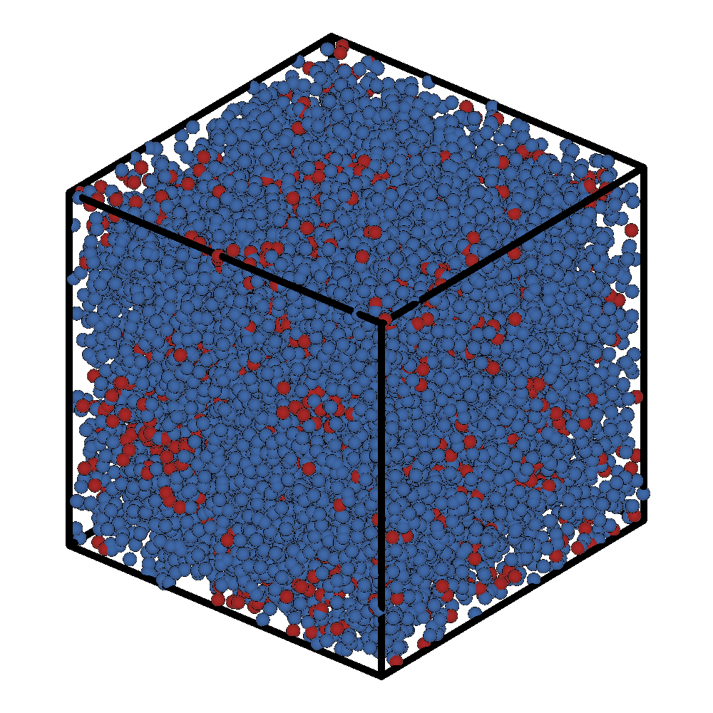
Initial Frame	Final Frame

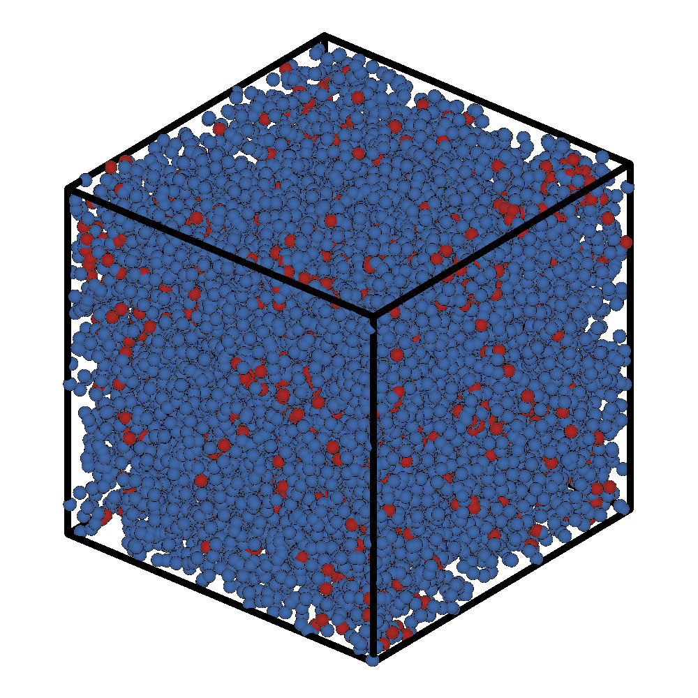
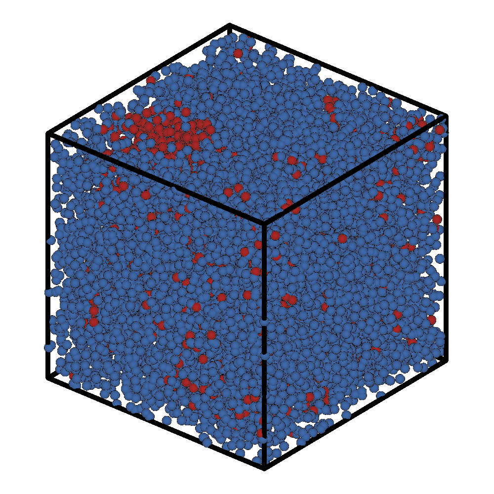
Even though we only ran 1000 steps, we see that a micelle has already formed in the top left corner of the box.

Another way to visualize this trajectory is to look at rhoA.dat and rhoB.dat. These files are written by LAMMPS (or more specifically, by fix_density_field) and contain the instantaneous density fields corresponding to the A and the B species.

rhoA = fk.read_from_file('rhoA.dat')
fk.plot(rhoA)

rhoB = fk.read_from_file('rhoB.dat')
fk.plot(rhoB)

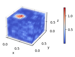
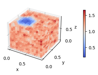
These visualizations make the micelle much easier to spot. If we re-visualize the SCFT densities from the start of the tutorial, we can see that fix_density_field has done a pretty good job.

density_fields = fk.read_from_file('density.dat')
fk.plot(density_fields)

Note: not plotting imaginary part of field 0
Note: not plotting imaginary part of field 1

Now that the MD simulation is pretty close to equilibrium, the typical next step is to turn off the bias and then run LAMMPS a bit longer to truly reach equilibrium. Once this step is done, you should have an equilibrated MD simulation with a density field consistent with an independent FTS run.

The next step is then up to you. Some possibilities:

• you can look at dynamics in MD

• you can analyze what individual chains are doing

• you can see if fluctuations destabilize a phase formed in SCFT

One of the big design goals of OpenFTS is to make running both FTS and MD simulations easy so that you (i.e. the user) can focus on the science. Hopefully now you’re ready to run both FTS and MD simulations with ease.

Mapping to HOOMD

Mapping to HOOMD is also easy.

fts.map_to_particle(simulation_type='hoomd',file_prefix='polymer')

Writing HOOMD input files:
  * gsdfile = polymer.gsd
  * jsonfile = polymer.json

This has generated three new files polymer.json, polymer.gsd and run-hoomd3.py. polymer.json contains the information needed to run a HOOMD simulation. These include bonded and non-bonded interaction parameters as well as information about the cell.

!head -n20 polymer.json

{
  "bond": {
    "kbond": [
      3.0,
      3.0,
      3.0
    ],
    "r0": [
      0.0,
      0.0,
      0.0
    ]
  },
  "config": {
    "cell": [
      11.430952132988164,
      11.430952132988164,
      11.430952132988164,
      0.0,
      0.0,

polymer.gsd contains the initial coordinates of all atoms in the system and the topology of the molecules (i.e. which atoms are bonded together). If you have fresnel installed, you can directly visualize this file using the script OpenFTS/python/tools/render-with-fresnel.py. Alternatively you can use VMD, Ovito or your visualization tool of choice.

run-hoomd3.py is the script you need to actually run a HOOMD simulation.

Unfortunately, its not currently possible to run HOOMD with a bias. One workaround is to first run LAMMPS with a bias and then convert the final frame of the LAMMPS dump trajectory into a gsd file that can be used as an initial configuration for a HOOMD run. OpenFTS contains a script that makes this conversion easy: OpenFTS/python/tools/lammpstrj_to_gsd.py

That it! You can now start running molecular dynamics simulations with the exact same model used in OpenFTS. Go forth!