Improving simulation performance
After defining an SCFT/FTS system, you may notice that your system is difficult to converge or equilibrate. Separately, you may also need your system to finish simulating as quickly as possible. For both of these scenarios the field updater parameters (\(\Delta t\), \(\{ \lambda_1, \lambda_2, ..., \lambda_n\}\)) need to be correctly chosen, and OpenFTS offers an effective approach to choose them via timestep optimization. In this tutorial, you will learn how to perform timestep optimization using the TimestepOptimizer class and its three different search methods.
Optimizing a 1D system with GridSearch
First let’s define a diblock melt system which we want to simulate with SCFT.
[1]:
import openfts

# Initialize an OpenFTS object.
fts = openfts.OpenFTS()

# Define the runtime mode, simulation cell, and field updater/layout.
fts.runtime_mode('serial')  # Run on CPU.
fts.cell(cell_scale=1.0, cell_lengths=[4.73846], dimension=1, length_unit='Rg')
fts.driver(dt=1.0, nsteps=1000, output_freq=250, stop_tolerance=1e-5, type='SCFT')
fts.field_updater(type='EMPEC', update_order='simultaneous',
                  adaptive_timestep=False, lambdas=[1.0, 1.0])
fts.field_layout(npw=[32], random_seed=1)

# Define the diblock blend model.
fts.model(Nref=50, bref=1.0, chi_array=[0.8], inverse_BC=1/20, type='MeltChiMultiSpecies')
fts.add_molecule(nbeads=50, nblocks=2, block_fractions=[0.5, 0.5],
                 block_species=['A', 'B'], type='PolymerLinear',
                 chain_type='discrete', volume_frac=1.0)
fts.add_species(label='A', stat_segment_length=1.0, smearing_length=0.15,
                smearing_length_units='Rg')
fts.add_species(label='B', stat_segment_length=1.0, smearing_length=0.15,
                smearing_length_units='Rg')

# Initialize the fields as phase separated.
fts.init_model_field(type='gaussians', height=1.0, ngaussian=1, width=0.1,
                     centers=[0], fieldname='mu_1')
fts.init_model_field(type='random', mean=0.0, stdev=1, fieldname='mu_2')

# Output the Hamiltonian and use default output names.
fts.add_operator(averaging_type='none', type='Hamiltonian')
fts.output_default()
This system microphase separates to form a lamellar phase with a unit cell length of about \(4.74 \: R_g\), and if we run a copy of this system with the trivial field updater parameters of \(\Delta t = \lambda_1 = \lambda_2 = 1.0\) we get the following outcome:
[2]:
import copy
fts_tmp = copy.deepcopy(fts)
fts_tmp.run()
================================================================
                           OpenFTS

OpenFTS version: heads/develop 7fd5b64 DIRTY
FieldLib version: remotes/origin/HEAD 9ce5644 CLEAN
Execution device: [CPU]
FieldLib precision: double
Licensee: Andrew Golembeski | aag99@drexel.edu | Expiration: 12/31/24
================================================================

Setup Species
  * label = A
  * stat_segment_length (b) = 1
  * smearing_length (a) = 0.15
  * smearing_length_units = Rg
  * charge = 0.000000
Setup Species
  * label = B
  * stat_segment_length (b) = 1
  * smearing_length (a) = 0.15
  * smearing_length_units = Rg
  * charge = 0.000000
Initialize Cell
  * dim = 1
  * length unit = Rg
  * cell_lengths = [4.738460 ]
  * cell_tensor:
4.73846
Initialize FieldLayout
  * npw = [32 ]
  * random_seed = 1
Setup MoleculePolymerLinear
  * chain_type = discrete
Setup ModelMeltChiMultiSpecies
  * bref = 1
  * Nref = 50
  * C = UNSPECIFIED
  * rho0 = UNSPECIFIED
  * chiN_matrix =
 0 40
40  0
  * compressibility_type = exclvolume
  * inverse_BC = 0.05
  * X_matrix =
[[4.47213595499958, 13.4164078649987],
 [13.4164078649987, 4.47213595499958]]
  * O_matrix (cols are eigenvectors) =
-0.707107  0.707107
 0.707107  0.707107
  * d_i = -8.94427191 17.88854382
Initialize MoleculePolymerLinear
  * Linear polymer has single chain:
    - type = discrete
    - nbeads = 50
    - discrete_type = Gaussian
    - sequence_type = blocks
    - nblocks = 2
    - block_fractions =  0.500000 0.500000
    - block_species =  A B
    - monomer_sequence (compact) =  A_25 B_25
    - monomer_sequence (long) = AAAAAAAAAAAAAAAAAAAAAAAAABBBBBBBBBBBBBBBBBBBBBBBBB
    - species_fractions =  0.5 0.5
  * volume_frac = 1
  * ncopies = UNDEFINED (since C undefined)
Initialize ModelMeltChiMultiSpecies
  * C/rho0 unspecified and all molecules specify volume_frac -> C/rho0 remain undefined (OK for SCFT).
  * exchange_field_names = 'mu_1' 'mu_2'
  * initfields = yes
    - set mu_1 as exchange field using gaussians
    - set mu_2 as exchange field using random 0+/-1
Initialize DriverSCFTCL
  * is_complex_langevin = false
  * dt = 1
  * output_freq = 250
  * output_fields_freq = 250
  * block_size = 250
  * field_updater = EMPEC
    - predictor_corrector = true
    - update_order = simultaneous
    - lambdas = 1.000000 1.000000
    - adaptive_timestep = false

  * field_stop_tolerance = 1e-05
Calculating Operators:
  * OperatorHamiltonian
    - type = scalar
    - averaging_type = none
    - save_history = true
Output to files:
  * scalar_operators  -> "operators.dat"
  * species_densities -> "density.dat"
                      ->  save_history = false
  * exchange_fields   -> "fields.dat"
                      ->  save_history = false
  * field_errors      -> "error.dat"

Running DriverSCFTCL
  * nsteps = 1000
  * resume = false
  * store_operator_timeseries = true

Starting Run.
Step:      1  H: 3.770749e-01 +0.000e+00i  FieldErr: 7.25e-01  TPS: 1470.21
Step:    250  H: 1.533078e+01 +0.000e+00i  FieldErr: 3.90e-02  TPS: 9903.94
Step:    500  H: 1.536908e+01 +0.000e+00i  FieldErr: 2.24e-03  TPS: 10887.25
Step:    750  H: 1.536916e+01 +0.000e+00i  FieldErr: 9.72e-05  TPS: 10609.34
SCFT converged in 932 steps to tolerance: 0.00 (fields)
* H = 15.3692 +0i
Run completed in 0.09 seconds (10289.30 steps / sec).
where we find that the system converges in 932 steps. Suppose we want to converge the system within 100 steps. Increasing \(\Delta t\), \(\lambda_1\), or \(\lambda_2\) will increase the magnitude of the field updates at every timestep, which generally results in faster convergence. However, if this magnitude is too great then the simulation will not converge. To find the largest magnitude possible, we can use the GridSearch search method of TimestepOptimizer.
[3]:
# Initialize a TimestepOptimizer object.
optimizer = openfts.TimestepOptimizer(fts)

# Set TimestepOptimizer's search method along with the method's keyword arguments.
optimizer.set_search_method('GridSearch', min_lambda=1.0, max_lambda=100.0,
                            points_per_lambda=40)

# Run TimestepOptimizer's search method parallelized over 12 processes with high verbosity.
optimizer.run(nprocs=12, verbosity=2)
Performing timestep optimization using GridSearch
Evaluating lambdas 1600 / 1600
TimestepOptimizer took 0.36 minutes in total
Optimal timestep: 1.0
Optimal lambdas: [34.55, 30.7]
GridSearch first creates a grid of different \(\left(\lambda_1, \lambda_2\right)\)’s with \(\Delta t\) held constant, and then evaluates each grid point. While this method can be computationally expensive, it is comprehensive. If we visualize the results of the search:
[4]:
optimizer.plot_results()
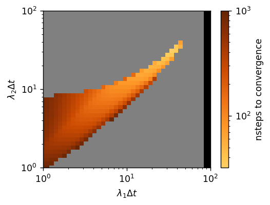
we can easily access the performance of the grid points evaluated. Gray-colored points did not converge before reaching the maximum number of steps (here 1000) and black-colored points diverged. We therefore have found many \(\left(\Delta t, \lambda_1, \lambda_2\right)\) which converge within 100 steps, meeting our goal! Through our search, we found the best field updater parameters to be \(\Delta t = 1.0\), \(\lambda_1 = 34.55\), \(\lambda_2 = 30.70\) which converges in 32 steps. Since each \(\lambda_i\) is multiplied by \(\Delta t\) in the field updater equation, this optimum is also equivalent to \(\Delta t = 10.0\), \(\lambda_1 = 3.455\), \(\lambda_2 = 3.070\).
Optimizing a 3D system with ManualSearch
Suppose now we want to optimize the previous system but instead it is 3D instead of 1D. We can use GridSearch again but now it will take significantly longer as 3D simulations have a higher computational cost. Because corresponding 1D and 3D SCFT systems can have similar performance under the same field updater parameters, another approach is to try the top 100 \(\left(\lambda_1, \lambda_2\right)\)’s of the 1D system in the 3D system with \(\Delta t\) held constant. We can perform this by using the ManualSearch search method. First, let’s create a file containing the top 100 \(\left(\lambda_1, \lambda_2\right)\)’s to evaluate.
[5]:
import numpy as np

# Get the lambdas evaluated and their performance as numpy arrays.
lambdas, performance, outcome, operators = optimizer.get_results()
lambdas = np.asarray(lambdas)
performance = np.asarray(performance)

# Get the top 100 lambdas (in order)
sort_indices = np.argsort(performance)
top_100_lambdas = lambdas[sort_indices[:100]]

# Write the top 100 lambdas to a file.
with open('lambdas.dat', 'w') as f:
    f.write('# Lambdas for ManualSearch.\n')
    for lam in top_100_lambdas:
        f.write(f'{lam[0]} {lam[1]}\n')
Now let’s define our 3D system and perform ManualSearch using these \(\left(\lambda_1, \lambda_2\right)\)’s. For 3D OpenFTS systems, running on a GPU greatly increases the speed of the simulation but let’s assume we only have access to a CPU. Let’s also assume that our goal is to find a simulation that can converge within 250 steps.
[6]:
# Create a copy of the 1D SCFT system.
fts_3D = copy.deepcopy(fts)

# Convert the copy to a 3D SCFT system.
fts_3D.params['cell']['cell_lengths'] = 3*[4.73846]
fts_3D.params['cell']['tilt_factors'] = 3*[0]
fts_3D.params['cell']['dimension'] = 3
fts_3D.params['fieldlayout']['npw'] = 3*[32]
fts_3D.params['model']['initfields']['mu_1']['center0'] = 3*[0]

# Change the maximum number of steps.
fts_3D.params['driver']['nsteps'] = 250

# Initialize a TimestepOptimizer object.
optimizer = openfts.TimestepOptimizer(fts_3D)

# Set TimestepOptimizer's search method along with the method's keyword arguments.
optimizer.set_search_method('ManualSearch', lambdas_file='lambdas.dat')

# Run TimestepOptimizer's search method parallelized over 12 processes with high verbosity.
optimizer.run(nprocs=12, verbosity=2)
Performing timestep optimization using ManualSearch
Evaluating lambdas 100 / 100
TimestepOptimizer took 9.63 minutes in total
Optimal timestep: 1.0
Optimal lambdas: [30.7, 27.28]
With ManualSearch, we reached our goal by finding that \(\Delta t = 1.0\), \(\lambda_1 = 30.70\), \(\lambda_2 = 27.28\) converges the 3D system within 250 steps. We can also clearly see how much longer 3D systems take to simulate than 1D systems on CPUs. Evaluating 100 \(\left(\lambda_1, \lambda_2\right)\)’s in the 3D system took us a little less than 10 minutes, while evaluating 1600 \(\left(\lambda_1, \lambda_2\right)\)’s in the 1D system only took us roughly a third of a minute.
Simulating a difficult system with BayesOptSearch
Occasionally you may find an OpenFTS system which does not converge or equilibrate with trivial field updater parameters. One such system is a homopolymer blend which undergoes macrophase separation, as defined below.
[7]:
# Initialize an OpenFTS object.
fts = openfts.OpenFTS()

# Define the runtime mode, simulation cell, and field updater/layout.
fts.runtime_mode('serial')  # Run on CPU.
fts.cell(cell_scale=1.0, cell_lengths=[4.0], dimension=1, length_unit='Rg')
fts.driver(dt=0.5, nsteps=1000, output_freq=250, stop_tolerance=1e-5, type='SCFT')
fts.field_updater(type='EMPEC', update_order='simultaneous',
                  adaptive_timestep=False, lambdas=[1.0, 1.0])
fts.field_layout(npw=[32], random_seed=1)

# Define the homopolymer blend model.
fts.model(Nref=100, bref=1.0, chi_array=[0.8], inverse_BC=1/100, type='MeltChiMultiSpecies')
fts.add_molecule(nbeads=100, nblocks=1, block_fractions=[1.0],
                 block_species=['A'], type='PolymerLinear',
                 chain_type='discrete', volume_frac=0.5)
fts.add_molecule(nbeads=100, nblocks=1, block_fractions=[1.0],
                 block_species=['B'], type='PolymerLinear',
                 chain_type='discrete', volume_frac=0.5)
fts.add_species(label='A', stat_segment_length=1.0, smearing_length=0.15,
                smearing_length_units='Rg')
fts.add_species(label='B', stat_segment_length=1.0, smearing_length=0.15,
                smearing_length_units='Rg')

# Initialize the fields as phase separated.
fts.init_model_field(type='gaussians', height=1.0, ngaussian=1, width=0.1,
                     centers=[0], fieldname='mu_1')
fts.init_model_field(type='random', mean=0.0, stdev=1, fieldname='mu_2')

# Output the Hamiltonian and use default output names.
fts.add_operator(averaging_type='none', type='Hamiltonian')
fts.output_default()
We can see that this system does not converge even if we increase the maximum number of steps by a factor of 10:
[8]:
fts_tmp = copy.deepcopy(fts)
fts_tmp.params['driver']['nsteps'] *= 10
fts_tmp.run()
================================================================
                           OpenFTS

OpenFTS version: heads/develop 7fd5b64 DIRTY
FieldLib version: remotes/origin/HEAD 9ce5644 CLEAN
Execution device: [CPU]
FieldLib precision: double
Licensee: Andrew Golembeski | aag99@drexel.edu | Expiration: 12/31/24
================================================================

Setup Species
  * label = A
  * stat_segment_length (b) = 1
  * smearing_length (a) = 0.15
  * smearing_length_units = Rg
  * charge = 0.000000
Setup Species
  * label = B
  * stat_segment_length (b) = 1
  * smearing_length (a) = 0.15
  * smearing_length_units = Rg
  * charge = 0.000000
Initialize Cell
  * dim = 1
  * length unit = Rg
  * cell_lengths = [4.000000 ]
  * cell_tensor:
4
Initialize FieldLayout
  * npw = [32 ]
  * random_seed = 1
Setup MoleculePolymerLinear
  * chain_type = discrete
Setup MoleculePolymerLinear
  * chain_type = discrete
Setup ModelMeltChiMultiSpecies
  * bref = 1
  * Nref = 100
  * C = UNSPECIFIED
  * rho0 = UNSPECIFIED
  * chiN_matrix =
 0 80
80  0
  * compressibility_type = exclvolume
  * inverse_BC = 0.01
  * X_matrix =
[[10, 18],
 [18, 10]]
  * O_matrix (cols are eigenvectors) =
-0.707107  0.707107
 0.707107  0.707107
  * d_i = -8 28
Initialize MoleculePolymerLinear
  * Linear polymer has single chain:
    - type = discrete
    - nbeads = 100
    - discrete_type = Gaussian
    - sequence_type = blocks
    - nblocks = 1
    - block_fractions =  1.000000
    - block_species =  A
    - monomer_sequence (compact) =  A_100
    - monomer_sequence (long) = AAAAAAAAAAAAAAAAAAAAAAAAAAAAAAAAAAAAAAAAAAAAAAAAAAAAAAAAAAAAAAAAAAAAAAAAAAAAAAAAAAAAAAAAAAAAAAAAAAAA
    - species_fractions =  1 0
  * volume_frac = 0.5
  * ncopies = UNDEFINED (since C undefined)
Initialize MoleculePolymerLinear
  * Linear polymer has single chain:
    - type = discrete
    - nbeads = 100
    - discrete_type = Gaussian
    - sequence_type = blocks
    - nblocks = 1
    - block_fractions =  1.000000
    - block_species =  B
    - monomer_sequence (compact) =  B_100
    - monomer_sequence (long) = BBBBBBBBBBBBBBBBBBBBBBBBBBBBBBBBBBBBBBBBBBBBBBBBBBBBBBBBBBBBBBBBBBBBBBBBBBBBBBBBBBBBBBBBBBBBBBBBBBBB
    - species_fractions =  0 1
  * volume_frac = 0.5
  * ncopies = UNDEFINED (since C undefined)
Initialize ModelMeltChiMultiSpecies
  * C/rho0 unspecified and all molecules specify volume_frac -> C/rho0 remain undefined (OK for SCFT).
  * exchange_field_names = 'mu_1' 'mu_2'
  * initfields = yes
    - set mu_1 as exchange field using gaussians
    - set mu_2 as exchange field using random 0+/-1
Initialize DriverSCFTCL
  * is_complex_langevin = false
  * dt = 0.5
  * output_freq = 250
  * output_fields_freq = 250
  * block_size = 250
  * field_updater = EMPEC
    - predictor_corrector = true
    - update_order = simultaneous
    - lambdas = 1.000000 1.000000
    - adaptive_timestep = false

  * field_stop_tolerance = 1e-05
Calculating Operators:
  * OperatorHamiltonian
    - type = scalar
    - averaging_type = none
    - save_history = true
Output to files:
  * scalar_operators  -> "operators.dat"
  * species_densities -> "density.dat"
                      ->  save_history = false
  * exchange_fields   -> "fields.dat"
                      ->  save_history = false
  * field_errors      -> "error.dat"

Running DriverSCFTCL
  * nsteps = 10000
  * resume = false
  * store_operator_timeseries = true

Starting Run.
Step:      1  H: 1.218931e-01 +0.000e+00i  FieldErr: 7.69e-01  TPS: 1124.29
Step:    250  H: 2.735070e+01 +0.000e+00i  FieldErr: 5.99e-01  TPS: 2504.39
Step:    500  H: 4.361468e+01 +0.000e+00i  FieldErr: 3.21e-01  TPS: 3042.24
Step:    750  H: 5.059678e+01 +0.000e+00i  FieldErr: 1.99e-01  TPS: 3047.10
Step:   1000  H: 5.344081e+01 +0.000e+00i  FieldErr: 1.34e-01  TPS: 2965.97
Step:   1250  H: 5.459605e+01 +0.000e+00i  FieldErr: 1.16e-01  TPS: 2938.48
Step:   1500  H: 5.496282e+01 +0.000e+00i  FieldErr: 3.30e-01  TPS: 3001.85
Step:   1750  H: 5.527022e+01 +0.000e+00i  FieldErr: 2.97e-01  TPS: 2971.07
Step:   2000  H: 5.516744e+01 +0.000e+00i  FieldErr: 5.73e-01  TPS: 2997.15
Step:   2250  H: 5.519802e+01 +0.000e+00i  FieldErr: 6.51e-01  TPS: 3057.75
Step:   2500  H: 5.459357e+01 +0.000e+00i  FieldErr: 7.41e-01  TPS: 3036.02
Step:   2750  H: 5.539947e+01 +0.000e+00i  FieldErr: 3.59e-01  TPS: 3008.34
Step:   3000  H: 5.605426e+01 +0.000e+00i  FieldErr: 4.18e-01  TPS: 3039.67
Step:   3250  H: 5.578217e+01 +0.000e+00i  FieldErr: 6.22e-01  TPS: 3058.59
Step:   3500  H: 5.473688e+01 +0.000e+00i  FieldErr: 7.91e-01  TPS: 2977.01
Step:   3750  H: 5.453012e+01 +0.000e+00i  FieldErr: 7.67e-01  TPS: 3037.10
Step:   4000  H: 5.568272e+01 +0.000e+00i  FieldErr: 3.19e-01  TPS: 3061.68
Step:   4250  H: 5.611712e+01 +0.000e+00i  FieldErr: 4.96e-01  TPS: 3062.00
Step:   4500  H: 5.550964e+01 +0.000e+00i  FieldErr: 6.80e-01  TPS: 2995.57
Step:   4750  H: 5.447476e+01 +0.000e+00i  FieldErr: 8.25e-01  TPS: 3065.51
Step:   5000  H: 5.483648e+01 +0.000e+00i  FieldErr: 6.37e-01  TPS: 3017.43
Step:   5250  H: 5.592160e+01 +0.000e+00i  FieldErr: 3.32e-01  TPS: 2945.99
Step:   5500  H: 5.604256e+01 +0.000e+00i  FieldErr: 5.61e-01  TPS: 2911.80
Step:   5750  H: 5.518283e+01 +0.000e+00i  FieldErr: 7.30e-01  TPS: 3017.41
Step:   6000  H: 5.436067e+01 +0.000e+00i  FieldErr: 8.39e-01  TPS: 2999.43
Step:   6250  H: 5.522179e+01 +0.000e+00i  FieldErr: 4.40e-01  TPS: 3008.42
Step:   6500  H: 5.606547e+01 +0.000e+00i  FieldErr: 4.04e-01  TPS: 2998.76
Step:   6750  H: 5.587658e+01 +0.000e+00i  FieldErr: 6.12e-01  TPS: 3045.76
Step:   7000  H: 5.484573e+01 +0.000e+00i  FieldErr: 7.76e-01  TPS: 3087.82
Step:   7250  H: 5.443600e+01 +0.000e+00i  FieldErr: 8.10e-01  TPS: 3034.33
Step:   7500  H: 5.557367e+01 +0.000e+00i  FieldErr: 3.37e-01  TPS: 2976.39
Step:   7750  H: 5.611922e+01 +0.000e+00i  FieldErr: 4.75e-01  TPS: 3041.38
Step:   8000  H: 5.562699e+01 +0.000e+00i  FieldErr: 6.58e-01  TPS: 3059.83
Step:   8250  H: 5.455745e+01 +0.000e+00i  FieldErr: 8.17e-01  TPS: 2994.06
Step:   8500  H: 5.469776e+01 +0.000e+00i  FieldErr: 7.07e-01  TPS: 3028.65
Step:   8750  H: 5.584267e+01 +0.000e+00i  FieldErr: 3.22e-01  TPS: 3018.73
Step:   9000  H: 5.608152e+01 +0.000e+00i  FieldErr: 5.40e-01  TPS: 2981.95
Step:   9250  H: 5.531412e+01 +0.000e+00i  FieldErr: 7.08e-01  TPS: 3032.14
Step:   9500  H: 5.438383e+01 +0.000e+00i  FieldErr: 8.42e-01  TPS: 3048.54
Step:   9750  H: 5.507128e+01 +0.000e+00i  FieldErr: 5.21e-01  TPS: 3048.05
Step:  10000  H: 5.602076e+01 +0.000e+00i  FieldErr: 3.74e-01  TPS: 2954.09
Run reached specified number of steps
Run completed in 3.34 seconds (2998.39 steps / sec).
and we find that the FieldErr is consistently fluctuating above 1e-01. In this scenario, our priority is converging the system and not the speed of convergence. Since we don’t need the costly comprehensive power of GridSearch and we don’t have any insightful guesses for ManualSearch, guessing field updater parameters in a statistically meaningful way is the next best strategy. This can be done with BayesOptSearch which uses Bayesian optimization to efficiently guess \(\left(\lambda_1, \lambda_2\right)\)’s.
[9]:
# Initialize a TimestepOptimizer object.
optimizer = openfts.TimestepOptimizer(fts)

# Set TimestepOptimizer's search method along with the method's keyword arguments.
optimizer.set_search_method('BayesOptSearch', min_lambda=1.0, max_lambda=100.0,
                            points_per_lambda=40, nlambdas=200)

# Run TimestepOptimizer's search method parallelized over 12 processes with high verbosity.
optimizer.run(nprocs=12, verbosity=2)
Performing timestep optimization using BayesOptSearch
Evaluating lambdas 200 / 200
TimestepOptimizer took 0.33 minutes in total
Optimal timestep: 0.5
Optimal lambdas: [24.24, 34.55]
Bayesian optimization works by first estimating the means and standard deviations of untried points by using a Gaussian processor regression (GPR) model, and then by acquiring untried points to sample through a so-called aquisition function. The aquisition function naturally seeks high performing points and is well-suited to our scenario. These features can be tuned through the keyword arguments of BayesOptSearch, but importantly let’s see how it performed.
[10]:
optimizer.plot_results()
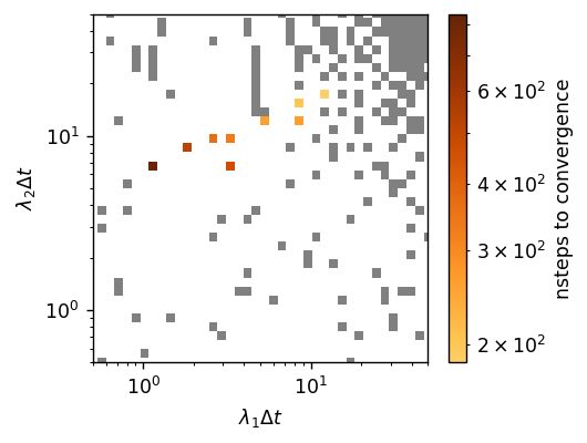
Based on the plot, BayesOptSearch found a few sets of field updater parmeters that converge! We can also see that BayesOptSearch choose most of its points around the best performing \(\left(\lambda_1, \lambda_2\right)\)’s. While this completes our task, for curiousity let’s see how far off BayesOptSearch was from the global optimum by using GridSearch.
[11]:
# Initialize a TimestepOptimizer object.
optimizer = openfts.TimestepOptimizer(fts)

# Set TimestepOptimizer's search method along with the method's keyword arguments.
optimizer.set_search_method('GridSearch', min_lambda=1.0, max_lambda=100.0,
                            points_per_lambda=40)

# Run TimestepOptimizer's search method parallelized over 12 processes with high verbosity.
optimizer.run(nprocs=12, verbosity=2)
Performing timestep optimization using GridSearch
Evaluating lambdas 1600 / 1600
TimestepOptimizer took 1.61 minutes in total
Optimal timestep: 0.5
Optimal lambdas: [27.28, 38.88]
[12]:
optimizer.plot_results()
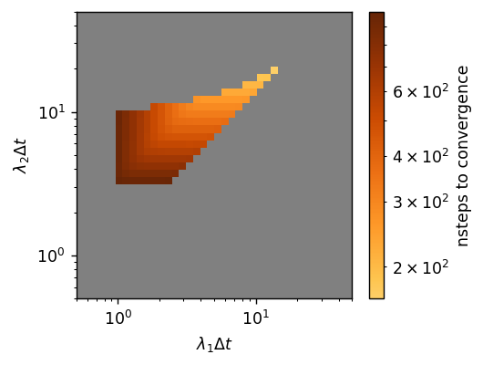
Compared to the global optimum, BayesOptSearch found field updater parameters that were slightly slower than GridSearch but in only one fifth of the time. Overall, GridSearch is well preferred when computationally tractable, but BayesOptSearch offers an alternative which can find convergent and performant field updater parameters in significantly less time.
TimestepOptimizer also offers additional run modifications for the search methods you’ve learned here. For more information, check out the Timestep Optimization page located under External Python Tools.